Merge Expert report CSVs

There are many ways to merge and dissect your data. This tutorial guides users through merging various Expert report CSVs.

How to merge tables with the VLOOKUP function

In this tutorial, we will use the users, groups and user2group reports to generate a single report that includes user IDs, group IDs, user names, emails, and group names. The process is relatively similar across many standard platforms (Excel, Numbers, Google Sheets). The example below uses VLOOKUP() in Excel to merge multiple tables.

Part 1: Download reports

If you are not familiar with where to download these reports, follow these links:

If you do not see an option to download these reports, contact Expert Support.

Part 2: Combine reports into a single CSV

Assume we are moving the groups data and user2group data to their own unique tabs in the users workbook.

Open the three CSV files.
Select the groups sheet.
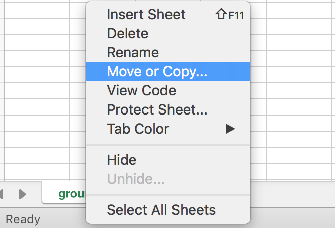
Right-click the groups tab (worksheet) and click Move or Copy.

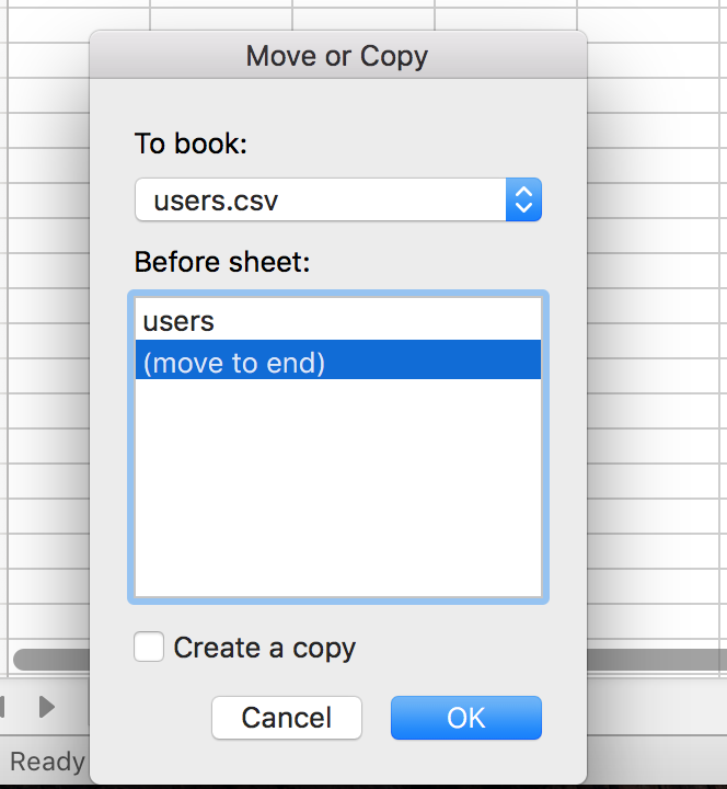
Reports -Merge - Excel move or copy.png

From the To book drop-down menu, select users.csv to specify the destination workbook.

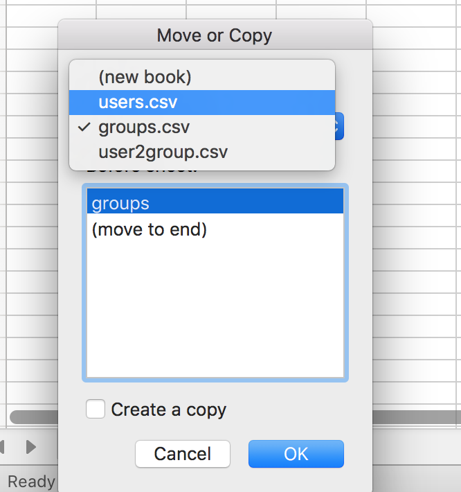
Reports -Merge - Excel move or copy select users.png

In the Before sheet field, select (move to end). This places the groups tab immediately after the users tab within the users workbook.

Reports -Merge - Excel move or copy move to end.png

Select the Create a copy checkbox if you do not want the sheets to be removed from the original workbook.
Click OK to move or copy the groups sheet from its original workbook to the users workbook.
Repeat this process to add the user2group sheet to the users workbook.
Make sure to save!

Part 3: Merge reports

Use VLOOKUP() to merge data from the three report into a single sheet that displays user ID, group ID, user name, email and group name.

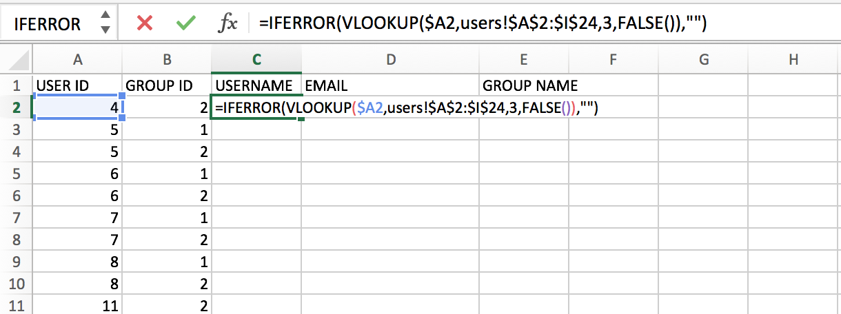
To the user2group sheet, add the headers USERNAME, EMAIL, and GROUP NAME.
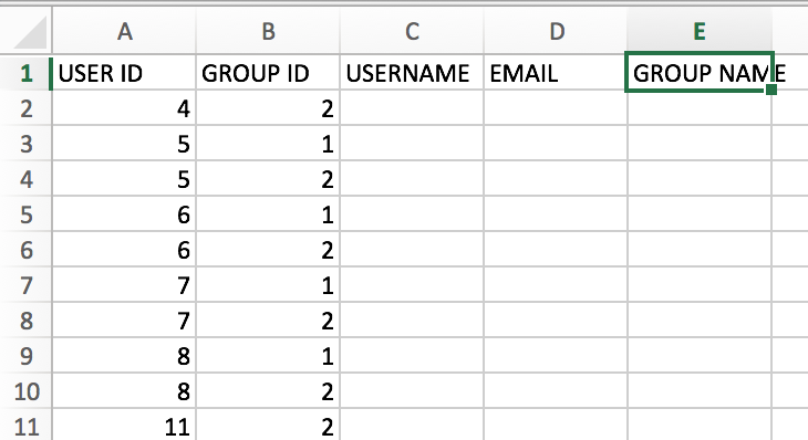
To look up usernames, add the following formula into cell C2: =IFERROR(VLOOKUP($A2,users!$A:$I,3,FALSE()),"").

VLOOKUP function explanation

The VLOOKUP()function allows you to look up a value referenced in another table and output that value. Its syntax looks as follows:

VLOOKUP(Lookup_value, Table_array, Col_index_num, [Range_lookup])

The table below explains the syntax of our VLOOKUP () function in =IFERROR(VLOOKUP($A2,users!$A:$I,3,FALSE()),"")

Reference	Purpose	In our example	Explanation
`Lookup_value`	Value you want to search for	`Lookup_value` is set to `$A2`	`$A2`is the first user ID listed in the user2group spreadsheet
`Table_array`	Range of cells that contains the data that you want to look up	`Table_array` is set to `users!$A:$I`	Includes all data from the users table
`Col_index_num`	number of the column in the `Table_array` that contains the data you’re looking for	`Col_index_num` is set to `3`	`3` represents the third column in the users table
`Range_lookup`	An optional argument in `VLOOKUP()` that can be either `True` or `False`. If `VLOOKUP()` is `True`, Excel tries to find an exact match for your `Lookup_value`. If Excel can’t find an exact match, Excel gives you the next largest value that is less than the `Lookup_value`.	`Range_lookup` is set to `FALSE()`	We only want to return exact results

IFERROR function explanation

The function IFERROR() traps and handles errors produced by other formulas or functions. Its syntax looks as follows:

IFERROR(Value, Value_if_error)

The table below explains the syntax of our IFERROR() function in =IFERROR(VLOOKUP($A2,users!$A:$I,3,FALSE()),"")

Reference	Purpose	In our example	Explanation
`Value`	Result of the associated function	`Value` is the `VLOOKUP()` function
`Value_if_error`	Value that replaces an erroneous value within that cell	`Value_if_error` is set to `""`	`""` replaces the `VLOOKUP()` output if it produces an error

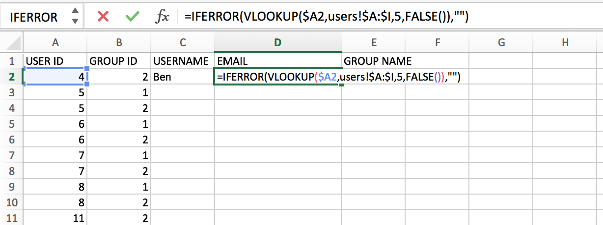
To look up emails, add the following formula into cell D2: =IFERROR(VLOOKUP($A2,users!$A:$I,5,FALSE()),"").

Reports -Merge - Excel look up emails.png

To look up group names, add the following formula into cell E2: =IFERROR(VLOOKUP($B2,groups!$A:$D,2,FALSE()),"")
To add the full list of usernames, emails and group names, select fields C2, D2,and E2 and drag them down to the bottom of the list (or double click the square at the bottom right-hand side of the highlighted selection).